Creating a scenario for the centralized / decentralized question

Creating a scenario for the centralized/decentralized question involves four steps:

1. Draw a sewer network.

2. Perform preliminary sizing of wastewater treatment plants.

3. Pre-select a treatment train for each wastewater treatment plant.

4. Create un scenario item.

For the same area, you can successively create as many scenarios as you wish.

Step 1: Pre-designing the sanitation sewer network (Sewer network Module)

Prerequisite

1. To have installed the pysewer library as explained in Installing external dependencies.

2. Have these 4 gis layers available:

• WWTP: vector layer containing all locations considered as potential discharge points (existing wastewater treatment plant or possible project location), type: point.

• buildings: vector layer containing the buildings to be connected, type: point (building centroids).

• roads: vector layer indicating the roads that can be used for connection, type: line.

• DEM: raster layer (.tif, .asc, .vrt) of the digital elevation model for the area of interest.

Attention

All 4 layers must be in the same CRS (coordinate reference system).

If you do not have these layers, see the page Obtaining and preparing geographic data for tips and explanations.

Using the module

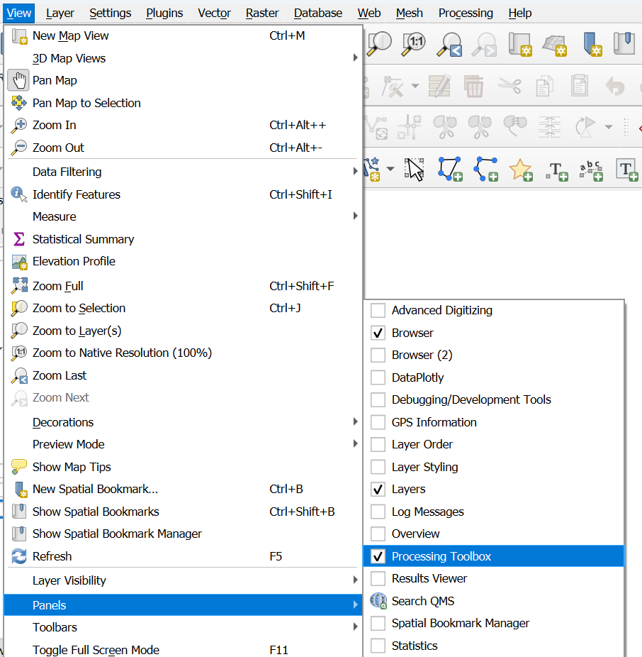
1. Search for elan in the Processing Toolbox and select Sewer network.

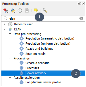
Tip

To display the Processing Toolbox panel if it does not appear in your workspace: View → Panels → Processing Toolbox. Or even easier: click on the gear icon just next to the sigma icon (top right a priori).

2. Fill in the four gis layers. Make sure the detected field for the Population (field) is correct.

Tip

For discharge points to be considered, you can first select the one(s) you want to consider among all the possible options and then tick Selected features only in the module. This option is also available for roads and buildings.

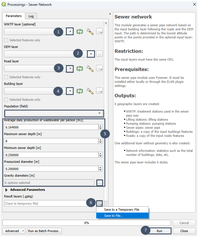
3. Adjust the various parameters (insert 5) in order to get the preliminary sizing of the network best suited to your context:

• average daily production of wastewater per person : [m³].

• maximum sewer depth: [m], depends on the geological context.

• minimum sewer depth: [m], generally conditioned by the risk of frost.

• pressurized diameter: [m], only one permitted diameter.

• gravity diameters: [m], to be chosen from the proposed options (0.1, 0.15, 0.2, 0.25, 0.3, 0.4, 0.6, 0.8 and 1.0). All 9 options may be considered, or only a subset of them.

Attention

It was observed that changes of maximum and minimum sewer depth default values are currently not taken into account (values stuck at 8 m and 0.25 m). The bug must be first corrected on pysewer before integration into Elan.

Note

You can also adjust other parameters pulling down the Advanced Parameters menu. Among them:

• peak load coefficient: [m³/s].

• minimum slope for sewer self-cleaning: [m/m].

• pipe roughness: [μm], depends on the material used for the pipes.

4. Indicate a location and name for the output .gpkg layer (marker 6), then run (marker 7).

5. After running the module, you obtain 1 .gpkg file containing 7 layers:

• WWTP (yellow square): point layer with the discharge point(s) considered for the simulation.

• Buildings : point layer with buildings considered for the simulation.

• Roads : line layer with the roads taken into account during the simulation.

• Lifting stations (green triangle): point layer containing the lifting stations of the pre-designed sewer network.

• Pumping stations (red triangle): point layer containing the pumping stations of the pre-designed sewer network (both private and non-private).

• Sewer pipes: line layer containing the pre-dimensioned sewer pipes.

• Network information: non-geometric layer gathering various metrics as attributes.

Note

WWTP, Buildings et Roads layers allow to keep track of simulation inputs. This is especially useful if you use the Selected features only option, but also not to lose the thread during scenarios exploration resulting of an iterative process (finer selection of buildings to connect, adding and/or deleting possible roads).

Each vector layer is characterized by attributes.

• WWTP: terrain elevation [m], gps coordinates (unique identifier for each discharge point), peak flow [m³/s], average daily flow [m³/day], inflow trench depths [m], inflow diameters [m], trench depth [m], inhabitants connected [number].

Note

At the Sewer network module output, the WWTP layer also has attributes that will be used as entries for the Processes module:

• outflow concentration targets: TSS outflow concentration target [mg/L], BOD₅ outflow concentration target [mg/L], TKN outflow concentration target [mg/L], COD outflow concentration target [mg/L], NO₃-N outflow concentration target [mg/L], TN outflow concentration target [mg/L], TP outflow concentration target [mg/L], e.coli outflow concentration target [UFC/100mL].

These attributes are to be filled manually for each discharge point according to your outflow concentration targets. Some of them can be set at NULL.

• inflow concentrations: TSS inflow concentration [mg/L], BOD₅ inflow concentration [mg/L], TKN inflow concentration [mg/L], COD inflow concentrationt [mg/L], NO₃-N inflow concentration [mg/L], TN inflow concentration [mg/L], TP inflow concentration [mg/L], inflow concentration [UFC/100mL].

These attributes are pre-filled with default values. They can be edited to better suit the user case. All of them must have a numerical value.

• Lifting stations: terrain elevation [m], peak flow [m³/s], average daily flow [m³/day], inhabitants connected [number], inflow trench depths [m], total static head [m].

• Pumping stations: terrain elevation [m], peak flow [m³/s], average daily flow [m³/day], inhabitants connected [number], inflow trench depths [m], total static head [m].

Note

Pumping stations can contain negative total static head for some of the stations. This is not a bug: it traduces that for such pumping stations, the pressurized section end point is lower than its starting point. In other terms : the pumping station acts as a siphon.

For example, here the pumping station is characterized by a total static head of -19.25 m.

• Sewer pipes: length [m], land profile [list of points sampled every 10 m], needs pump [boolean], pressurized [boolean], sewer profile [list of points sampled every 10 m], mean trench depth [m], diameter [m], peak flow [m³/s], WWTP coordinates [WWTP discharge point identifier].

• Network information: total buildings [count], pressurized sewer lenght [linear meters], gravity-driven sewer lenght [linear meters], pumping stations number [count], lifting stations number [count], simulation datetime [datetime].

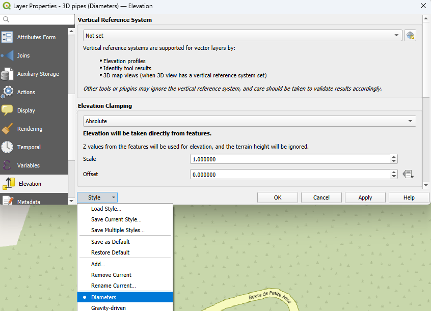
Several styles are available for the Sewer pipes layer.

• Diameters: categorized symbology on the diameter attribute to visualize the distribution of diameters within the sewer network.

• Peak flow: categorized symbology on the peak flow attribute to view variation in peak flow along the sewer network segments.

• Gravity-driven: categorized symbology on the pressurized attribute to easily distinguish gravity-driven sections from pressurized sections. This is the default style in the Sewer network module output.

• Depth: categorized symbology on the mean trench depth attribute to better visualize variations in depth within the sewer network.

• Flow direction: symbology with arrows to better understand the flow direction inside the sewer network.

• Sub-networks: categorized symbology on the WWTP coordinates attribute to clearly identify the different networks in case the area is connected to several plants (decentralized management).

Attention

If you save simulation output as a temporary layer and then save it afterward, the proposed formatting (symbologies, styles, layer names) will not be preserved. Only saving a file directly when launching the module and saving it in your QGIS project ensures that they are retained.

Results exploration (Longitudinal sewer profile module)

To explore the preliminary sizing proposed by the Sewer network module, in addition to the different styles available for the Sewer pipes layer, the Longitudinal sewer profile module and visualization of its outputs using QGIS’s Elevation Profile tool allow you to view the underground profile of a sequence of pipes.

Prerequisite

Have a Sewer pipes layer generated by the Sewer network module.

Using the module

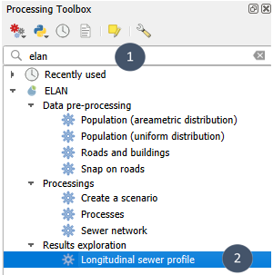
1. Search for elan in the Processing Toolbox and select Longitudinal sewer profile.

2. Provide the sewer pipes layer (marker 1), choose a location and a name for the output file (marker 2), then run (marker 3).

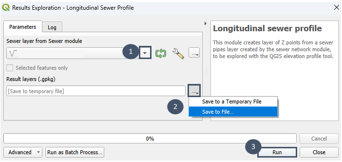
3. The module generates 1 .gpkg file containing 3 layers:

• Land profile: point layer containing a sampling of DEM values (ground elevation) along the pipe profile.

• Sewer profile: point layer whose points overlap with those of the Land profile layer in the XY plane, but correspond to pipe elevation.

• 3D pipes: Z-enabled line layer created from a sampling of the Sewer pipes layer (retains styles and attributes).

Visualization

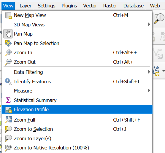
1. To display a pipe profile in an XZ plane, start by opening the Elevation Profile tool: View → Elevation Profile.

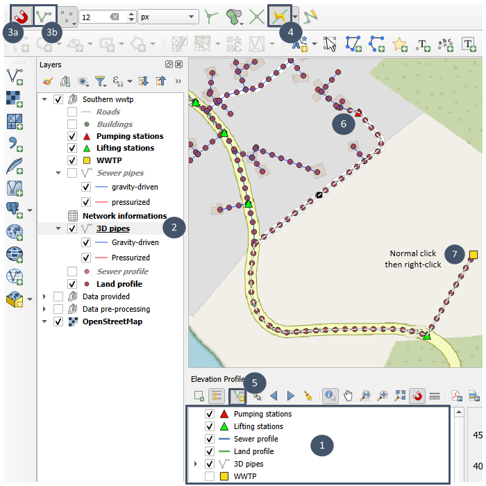
2. In the Elevation Profile window, tick the layers you want to appear in your section. For example: Lifting stations, Pumping stations, Land profile, Sewer profile and 3D pipes (marker 1).

3. Select the pipes whose underground profile you want to display. To do this:

• Select the 3D pipes layer (marker 2).

• Enable snapping (marker 3a) on the active layer (marker 3b).

Tip

If Enable Snapping is not visible : enable it via View → Toolbars → Snapping Toolbar.

• Enable tracing (marker 4).

• In the Elevation Profile window, click the Capture Curve icon (marker 5).

• Click the first point (marker 6).

• Click the last point (marker 7).

• Then right-click to activate the trace between these two points (marker 7).

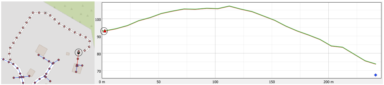
4. Your profile will then appear in the Elevation Profile window.

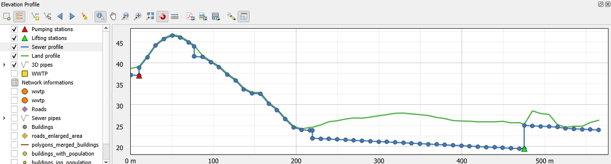
This view shows the terrain relief and the profile of sampled pipes. It gives a good visualization of drops at manholes. However, it does not clearly distinguish between gravity and pressurized sections, nor does it omit points arriving from other alignments at manholes.

5. By unchecking Sewer profile, you obtain this view.

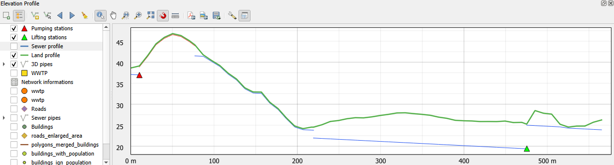
Here, the drops at manholes are not shown (discontinuities in the trace). On the other hand, pressurized sections (in red) are clearly distinguished from gravity sections (in blue), and points arriving from other alignments do not interfere with interpretation of the profile.

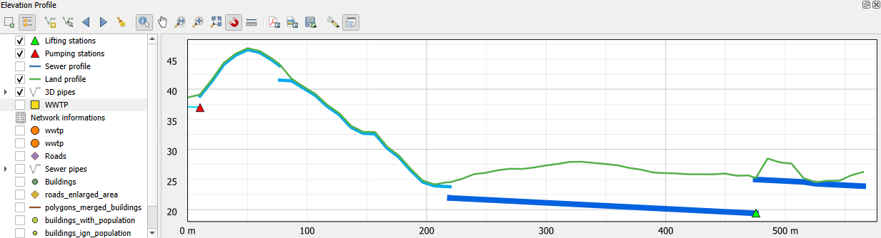
6. You can also obtain a view by diameters.

To do this:

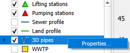
• Right-click on 3D pipes in the Elevation Profile window and select Properties.

• In the window that opens, click Style (at the bottom) and select Diameters.

Tip

You can also obtain the diameter-based view from the Layers panel:

• Right-click on 3D pipes.

• Go to Styles.

• Choose Diameters.

• Untick and then retick the 3D pipes layer in the Elevation Profile window so the new style is applied.

Step 2: Preliminary sizing of the WWTP(s) (Processes module)

To complete your scenario, the next step is to size the wastewater treatment plant(s) that serve as discharge points of your sewer network.

The Processes module allows you, for each wastewater treatment plant, to test and pre-size different treatment trains based on constructed wetlands (CW).

The treatment trains can be composed of 1 to n stages (maximum n = 3) and may involve different processes: French vertical flow treatment wetland (VdNS1), vertical flow treatment wetland using sand (VdNS2), French vertical flow treatment wetland with a saturated bottom layer (VdNSS).

Prerequisite

1. To have installed the wetlandoptimizer library as explained in Installing external dependencies.

2. Have a point layer with the location(s) of the possible wastewater treatment plants.

This layer must contain a minima 18 attributes: gps coordinates, average daily flow [m3/j], TSS inflow concentration [mg/L], BOD₅ inflow concentration [mg/L], TKN inflow concentration [mg/L], COD inflow concentration [mg/L], NO₃-N inflow concentration [mg/L], TN inflow concentration [mg/L], TP inflow concentration [mg/L], e.coli inflow concentration [UFC/100mL], TSS outflow concentration target [mg/L], BOD₅ outflow concentration target [mg/L], TKN outflow concentration target [mg/L], COD outflow concentration target [mg/L], NO₃-N outflow concentration target [mg/L], TN outflow concentration target [mg/L], TP outflow concentration target [mg/L], e.coli outflow concentration target [UFC/100mL].

For the outflow concentration targets, 3 must necessarily be filled with a numerical value strictly greater to 0: TSS outflow concentration target [mg/L], BOD₅ outflow concentration target [mg/L], COD outflow concentration target [mg/L]. The others can be set to NULL depending on your context (all or some of them).

Attention

Currently, the optimization performed by wetlandoptimizer does not take into account outflow concentration targets relative to total phosphorus (TP) and e.coli (default values considered: NULL). This will be integrated in a future version.

This layer can be obtained as output from the Sewer network module. In that case, average daily flow and GPS coordinates are automatically filled. The outflow concentration targets attributes are present but must be filled manually according to your discharge requirements. Inflow concentrations are pre-filled with default values but they can be edited to better suit your context.

3. Have defined and saved the available surface areas for each wastewater treatment plant in a polygon layer.

This is optional and does not affect pre-sizing itself: it simply helps you identify which treatment trains, among those that meet your discharge constraints, are also compatible with your surface area constraints.

Using the module

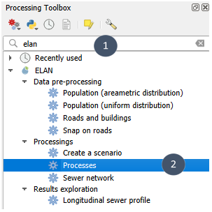
1. Search for elan in the Processing Toolbox and select Processes.

2. Indicate whether your zone is in a Temperate or Tropical climate (marker 1). This choice impacts the pre-sizing of treatment trains in terms of surface area and volume (smaller surface area and volume under tropical climate).

Note

Choose Tropical if the minimum temperature is greater than or equal to 18 °C all year round.

For more information on proper consideration of tropical climate in the design of constructed wetlands:

Lombard-Latune and Molle (2017). Constructed wetlands for domestic wastewater treatment under tropical climate: Guideline to design tropicalized systems. Guides and protocols. 72 pages. Agence française de la biodiversité.

3. Provide the WWTP layer (marker 2) and, optionally, the available surface areas layer (marker 3).

4. Make sure the detected fields for GPS coordinates and daily inflow are correct (insert 4).

Note

Unfolding Advanced parameters, you can also make sure that inflow concentrations and outflow concentration targets for the various pollutants were correctly auto-detected.

5. For the maximum number of stages, we recommend leaving the default value of 3 (insert 4).

6. Choose a save location and name for the output file (marker 5) and then run (marker 6).

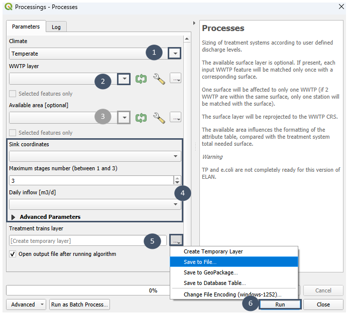
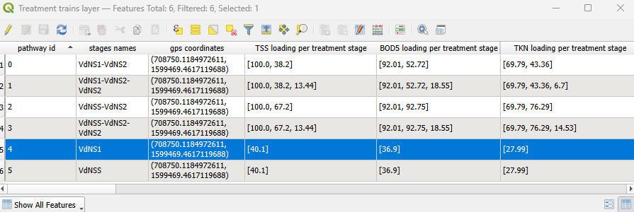
7. After execution, you obtain a layer called Treatment trains layer (point layer).

This layer gathers all the treatment trains tested during optimization (a feature = a treatment train). Each feature is characterized by various attributes:

• pathway id: numerical identifier of the pre-sized treatment train.

• stages names: details of the treatment train (process stage 1 - … - process stage n).

• gps coordinates: WWTP identifier for which the treatment train was pre-sized.

• TSS loading per treatment stage [%]: TSS loading rate per stage [stage 1, …, stage n].

• BOD5 loading per treatment stage [%]: BOD₅ loading rate per stage [stage 1, …, stage n].

• TKN loading per treatment stage [%]: TKN loading rate per stage [stage 1, …, stage n].

• COD loading per treatment stage [%]: COD loading rate per stage [stage 1, …, stage n].

• hydraulic loading rate [%]: hydraulic loading rate per stage [stage 1, …, stage n].

• available surface [m²]: calculated from the polygon layer provided when launching the module (optional layer).

• total surface [m²]: total surface of the treatment train (sum of surface areas of stages 1 to n).

The total surface area value determines its formatting: if it is less than or equal to the available surface area, the cell appears green; otherwise, it appears red.

• surface per treatment stage [m²]: details of surface areas for each stage [stage 1, …, stage n].

• total volume [m³]: total volume of the treatment train (sum of volumes of stages 1 to n).

• saturated depth per stage [m]: details of saturated depth for each stage [saturated depth stage1,…, saturated depth stage n].

This value is zero for VdNS1 and VdNS2 processes, which have no saturated layer.

• unsaturated depth per stage [m]: details of unsaturated depth for each stage [unsaturated depth stage1,…, unsaturated depth stage n].

• TSS outflow concentration [mg/L]: TSS concentration at the outlet of the treatment train.

• BOD5 outflow concentration [mg/L]: BOD₅ concentration at the outlet of the treatment train.

• TKN outflow concentration [mg/L]: TKN concentration at the outlet of the treatment train.

• COD outflow concentration [mg/L]: COD concentration at the outlet of the treatment train.

• TN outflow concentration [mg/L]: TN concentration at the outlet of the treatment train.

• NO3-N outflow concentration [mg/L]: NO₃-N concentration at the outlet of the treatment train.

• TP outflow concentration [mg/L]: TP concentration at the outlet of the treatment train.

• e.coli outflow concentration [UFC/100mL]: e-coli concentration at the outlet of the treatment train.

• TSS deviation [mg/L] : deviation of TSS outflow concentration relative to target.

• DBO5 deviation [mg/L] : deviation of BOD₅ outflow concentration relative to target.

• TKN deviation [mg/L] : deviation of TKN outflow concentration relative to target.

• COD deviation [mg/L] : deviation of COD outflow concentration relative to target.

• TN deviation [mg/L] : deviation of TN outflow concentration relative to target.

• NO3-N deviation [mg/L] : deviation of NO₃-N outflow concentration relative to target.

• TP deviation [mg/L] : deviation of TP outflow concentration relative to target.

• COD deviation [mg/L] : deviation of COD outflow concentration relative to target.

Deviations are formatted based on their value : green if lower than or equal to 0, red if greater than 0. They give information regarding treatment train compliance with outflow concentration target specified as inputs: green = compliant, red = non-compliant.

• TSS normalized [-] : normalized value of TSS achieved outflow concentration relative to target.

• DBO5 normalized [-] : normalized value of BOD₅ achieved outflow concentration relative to target.

• TKN normalized [-] : normalized value of TKN achieved outflow concentration relative to target.

• COD normalized [-] : normalized value of COD achieved outflow concentration relative to target.

• TN normalized [-] : normalized value of TN achieved outflow concentration relative to target.

• NO3-N normalized [-] : normalized value of N-NO₃ achieved outflow concentration relative to target.

• TP normalized [-] : normalized value of TP achieved outflow concentration relative to target.

• e.coli normalized [-] : normalized value of e.coli achieved outflow concentration relative to target.

• surface normalized [-] : normalized value of required surface relative to available surface area.

If the normalized value is lower than or equal to 1, then the constrainst is satisfied (outflow concentration target or available surface area). If not, it exceeds this constraint.

Note

For optional parameters (outflow concentration targets of some pollutants, available surface area), if no value is specified, their deviation and normalized values are not calculated (NULL).

Important

Among features of the Treatment trains layer , only treatment trains with “green” deviations meet the outflow concentration targets specified as inputs of the module.

The sequence of processes (stages names) differs from one treatment train to another.

For each treatment train, in addition to the achieved outflow concentrations, geometric characteristics are provided (total surface, surface per stage, total volume, saturated depth, unsaturated depth), along with performance characteristics (loading rates per stage for different pollutants and hydraulic loading rate per stage) and compliance indicators based on specified constraints (deviations, normalized values).

The per-stage loading rates can be useful indicators depending on future projections for the area, and can help guide your choice of treatment train. For example, if a high population increase is expected in the area, it would be better to choose a treatment train that is not already operating at maximum pollutant loads in the current configuration.

Step 3: Pre-selecting a treatment train for each discharge point

Among the pre-sized treatment trains, some meet the required outflow concentrations (deviations in green), others non (deviations in red), with their own surface requirements that can exceeds the available surface area (total surface in red if avaible surface was specified).

Graphical representations (bar plot and radar plot) were included to Elan for easier visualization of the Processes module ‘s outputs. They make it easier to identify the respective strengths and weaknesses of each suggested treatment trains.

To use these graphical representations, you need to:

• Have installed the Data Plotly plugin as explained in Installing QGIS third-party plugins.

• Have a layer Treatment trains layer (output of the Processes module).

• If your Treatment trains layer layer has several discharge points, to have selected one of them.

Important

The radar plot and the bar plot aim to compare several possible treatment trains for a same discharge point. If your Treatment trains layer contains multiple discharge points and you forget to select only one of them, an error message will appear when trying to visualize one of the two plots.

Radar plot

Compliance with required outflow concentrations and available surface are two fairly obvious criteria that will allow you to pre-select a treatment train for each discharge point. The radar plot integrated to Elan allows to graphically visualize the several treatment trains based on these criteria and thus facilitate their comparison.

To do this:

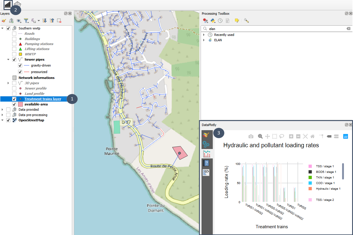
1. Click on your layer Treatment trains layer in the Layers panel (marker 1).

2. Click on the button with a radar plot icon (marker 2).

3. A DataPlotly window pops up in the lower right side of you screen (below Processing Toolbox, marker 3).

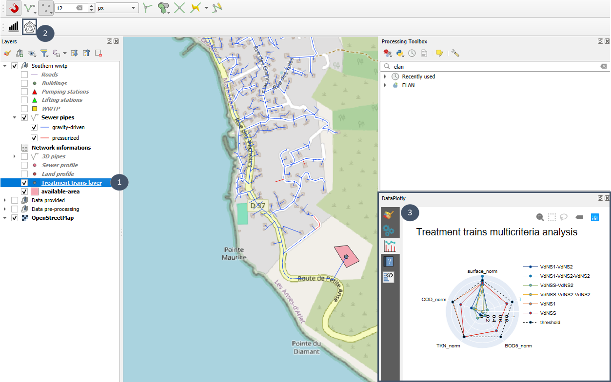
4. You can expand or move the window to better see the plot.

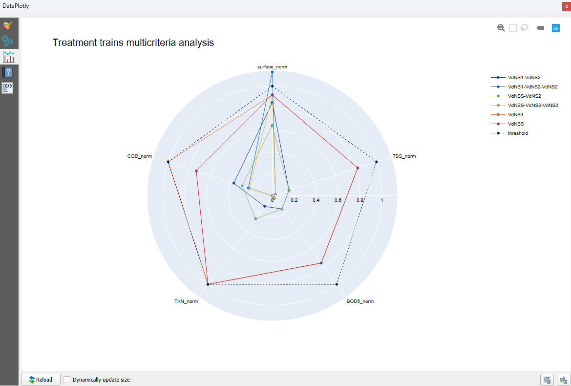
The radar plot axes match the constraints specified by the user in the WWTP layer (output of the Sewer network) when editing it before using the Processes module. In this example, the user stated constraints (outflow concentration targets) for 4 pollutants (TSS, COD, DBO₅ and TKN) and for the surface available to implement a treatment train (polygon layer given as input for the Processes module).

The dotted line represents the constraints : a point below this threshold indicates that the constraint for the axis is satisfied when a point above traduces a non-compliance of the treatment train for this criteria.

By default, all possible treatment trains for the considered discharge point appear on the radar plot. If you want to see only some of them, you just have to select them in the attribute table and click again on the radar plot button.

Bar plot

Pollutant loading rates and hydraulic loading rate may also help you in pre-selecting appropriate treatment trains. The bar plot integrated to Elan allows you to graphically visualize these attributes.

To do this:

1. Click on your layer Treatment trains layer in the Layers panel (marker 1).

2. Click on the button with a bar plot icon (marker 2).

3. A DataPlotly window pops up in the lower right side of you screen (below Processing Toolbox, marker 3).

4. You can expand or move the window to better see the plot.

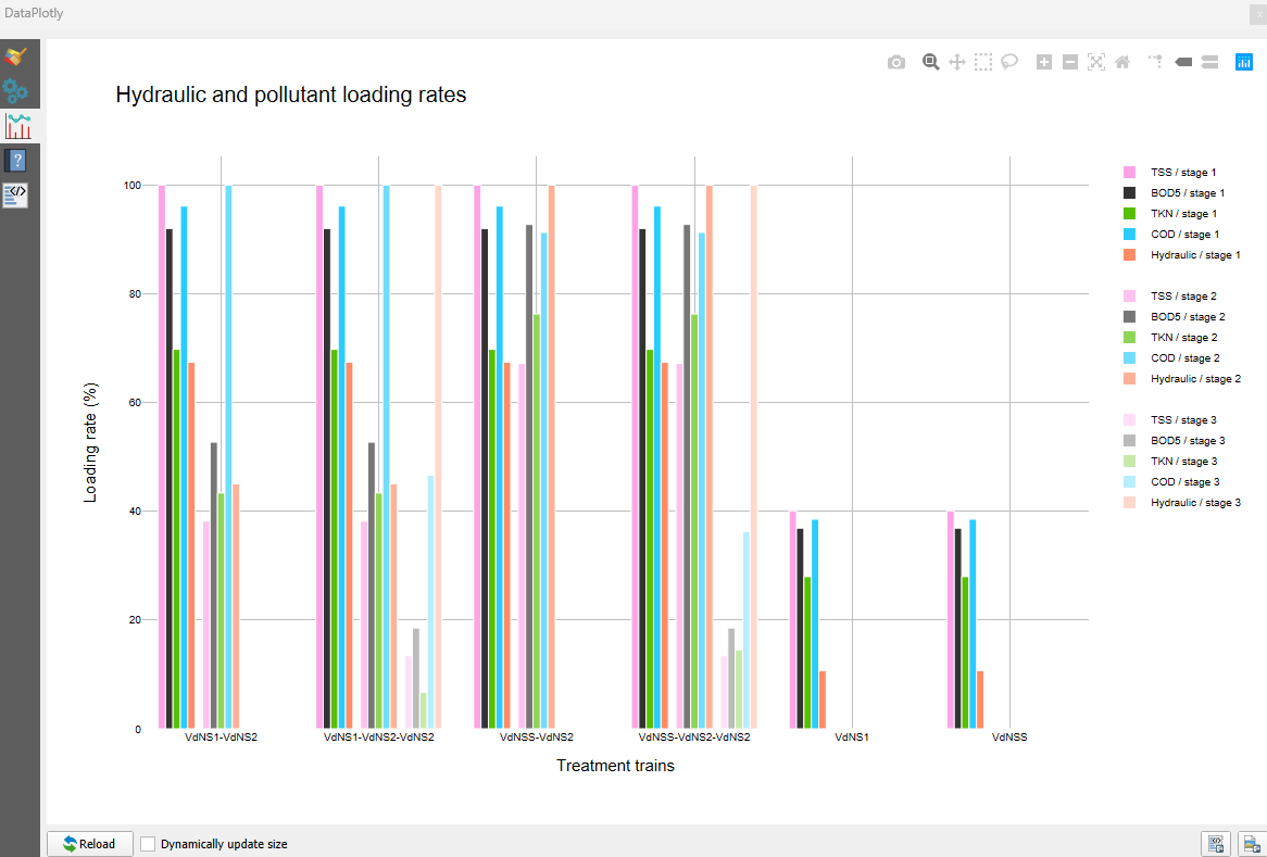
For each treatment train, this plot shows per stage the TSS, BOD₅ , TKN and COD loading rates along with the hydraulic loading rate. A one stage treatment train appears with only one “block” gathering all the loading rates relative to “stage 1” (colors of maximum intensity), while a three stages treatment train contains 3 “blocks” with the loading rates for “stage 1”, “stage 2” and “stage 3” (colors of decreasing intensity : maximum for “stage 1” and minimum for “stage 3”).

The bar plot allows you to identify the element.s that were limiting during the treatment train optimisation (100 % loading rate) and have a quick idea whether the treatment train is adaptative or not in case of evolution of the context (increase of population for instance).

By default, all possible treatment trains for the considered discharge point appear on the bar plot. If you want to see only some of them, you just have to select them in the attribute table and click again on the bar plot button.

Step 4: Creation of a scenario item (Create a scenario module)

The Create a scenario module allows you to create a scenario item gathering pre-sizing of the sewer network and of its associated treatment trains (1 per discharge points).

The scenario item is a geopackage. Based on this file, the scenario could then be assessed by the Assessment module.

Prerequisite

1. Have a Sewer pipes layer generated by the Sewer network module.

2. To have achieved preliminary design of treatment trains for each discharge points considered in this Sewer pipes` layer using the Processes module (Treatment trains layer layer)

3. To have chosen one treatment train option for each discharge points among all the pre-sized ones.

Using the module

1. Open the attribute table of your Treatment trains layer and select one treatment train per discharge point. For example here, the VdNS1 treatment train (1 unique treatment train selected because only 1 discharge point in this scenario).

2. Search elan in the Processing Toolbox and select Create a scenario.

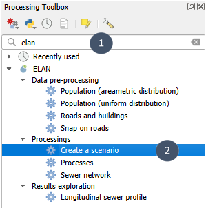
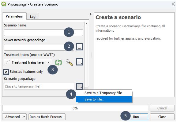
3. Give a name to your scenario (marker 1), specify the Sewer pipes layer to be considered (marker 2), indicate the Treatment trains layer and compulsory tick Selected features only (marker 3) to consider only the pre-selected treatment train(s).

4. State a name and a save location for the output file (marker 4), then run (marker 5).

5. The module generates 1 .gpkg file with 9 layers:

• 7 layers from the Sewer network module.

• 1 Treatment trains layer layer with the selected treatment trains.

• 1 non geometric layer metadata with a unique identifier for later comparison with other scenarios.

Important

The output geopackage is not loaded in the QGIS project. It is saved at the specified location, ready to be opened in a new QGIS project for future assessment and comparison.