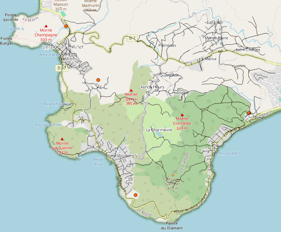
Petite Anse example

This tutorial is based on Petite Anse case and details all the steps to be implemented to create a scenario for the centralized / decentralized question, from obtaining and preparing geographical data to creating a scenario item.

It can be followed step by step to get started with Elan before using the plugin on your own case. An exercise to create another scenario for Petite Anse area is suggested at the end of this tutorial.

Obtaining and preparing geographic data

Prerequisite: Display a base map (here OpenStreetMap)

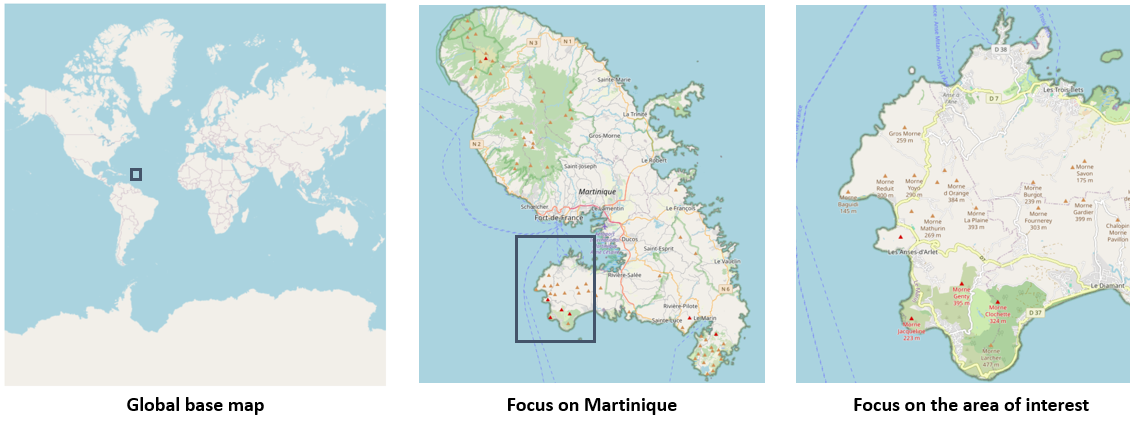
To locate the area, display the OpenStreetMap basemap:

• Go to the Browser panel.

Tip

If the Browser panel is not visible: enable it via View → Panels → Browser.

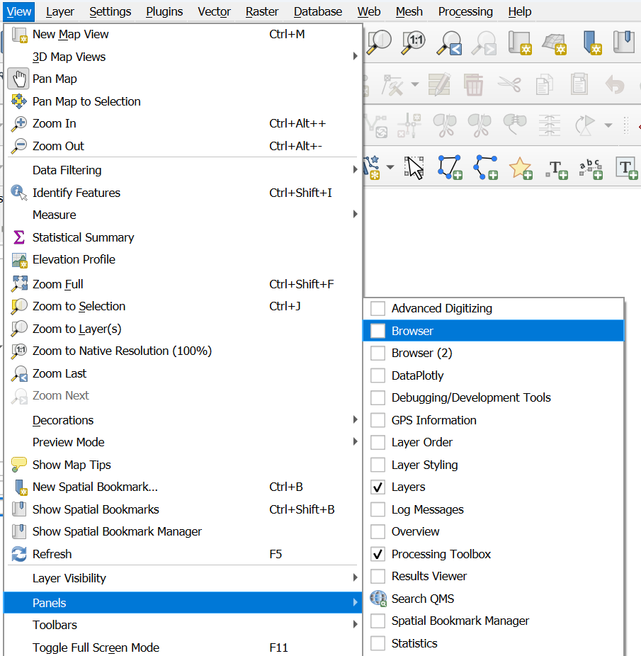
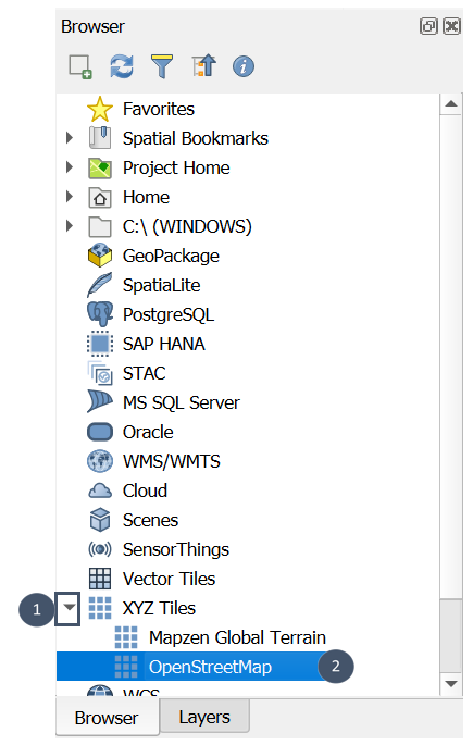
• Search for the XYZ Tiles category (marker 1).

• Expand and double-click on OpenStreetMap (marker 2).

• Locate the area on the OpenStreetMap basemap displayed in your map view.

Note

For more details on available basemaps in QGIS, refer to QGIS documentation (For users section).

Step 1: Get the Digital Elevation Model (DEM)

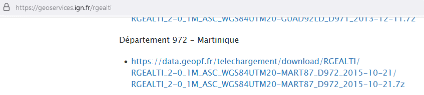
1. Download the 5 m DEM for Martinique from RGE ALTI®.

2. Identify the DEM tiles covering your area of interest by loading them into your QGIS project (via the Browser panel).

Tip

Here a grid associated to the DEM tiles is available (dalles.shp in 3_SUPPLEMENTS_LIVRAISON). Loading it into QGIS via the Browser panel (marker 1) allows you a quicker identification of the tiles of interest.

All you have to do is to select the tiles covering your area (markers 2 and 3) and do Open Attribute Table (Selected Features) (marker 4) to access directly their names (attribute NOM DALLE).

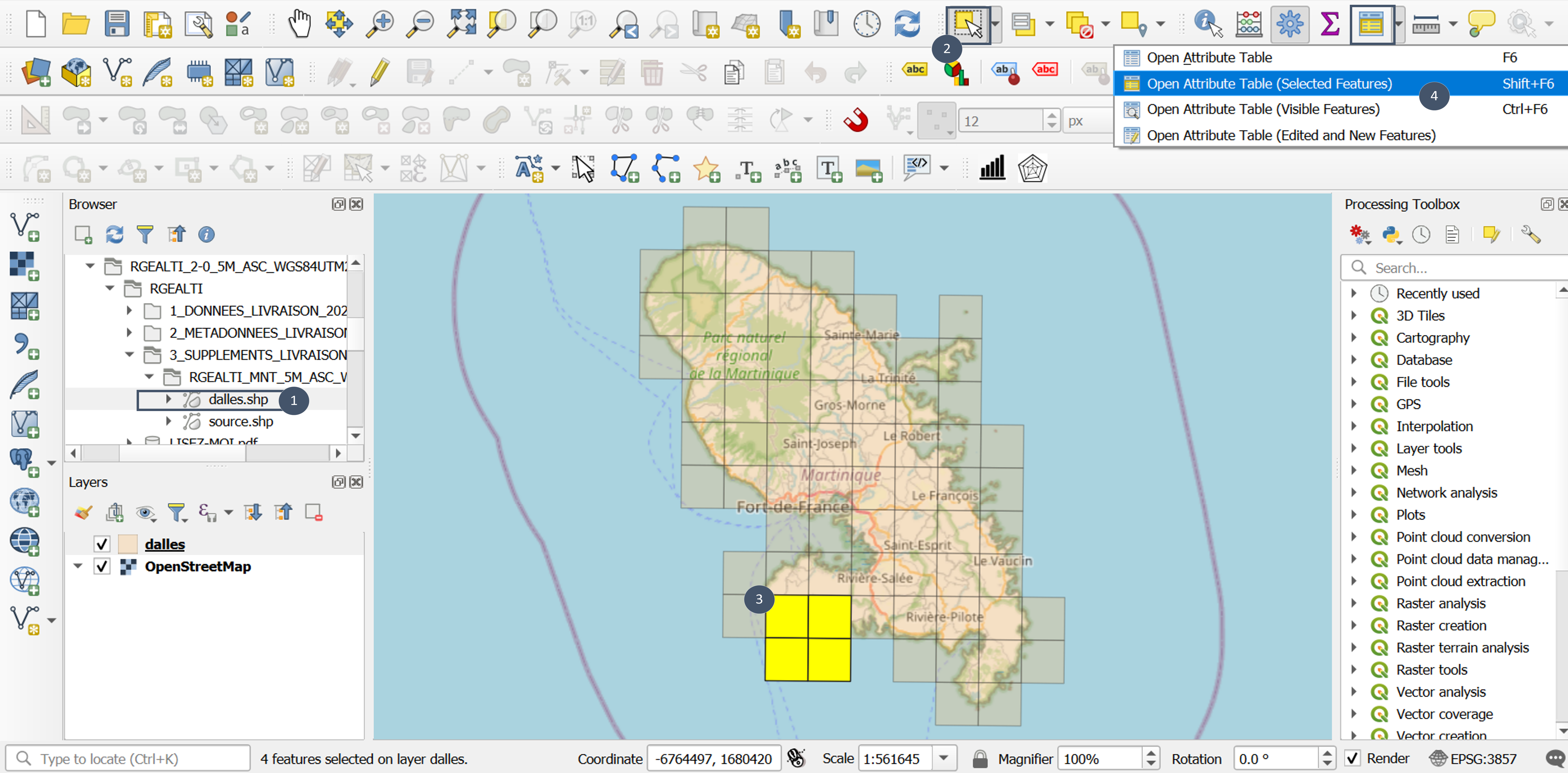
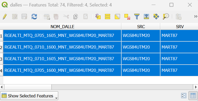
In this case, four tiles cover the area: RGEALTI_MTQ_0705_1600_MNT_WGS84UTM20_MART87, RGEALTI_MTQ_0710_1600_MNT_WGS84UTM20_MART87, RGEALTI_MTQ_0705_1605_MNT_WGS84UTM20_MART87 and RGEALTI_MTQ_0710_1605_MNT_WGS84UTM20_MART87.

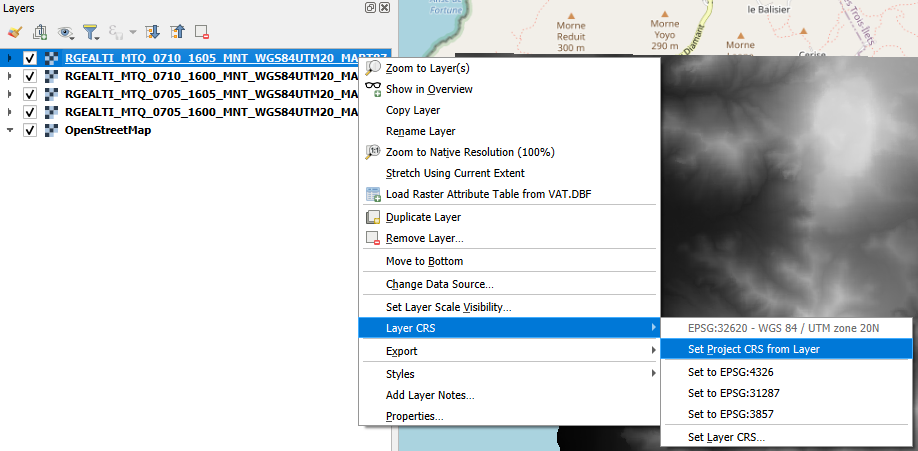
3. Identify the associated CRS (Coordinate Reference System). It is usually indicated in the file names: here WGS184UTM20, i.e., EPSG:32620 – WGS 84 / UTM zone 20N in QGIS.

4. Assign this CRS to the 4 tiles (no automatic detection).

Tip

Make the DEM’s CRS your project CRS: choose it when creating new layers and reproject imported vector layers into this CRS using QGIS’s Reproject layer tool.

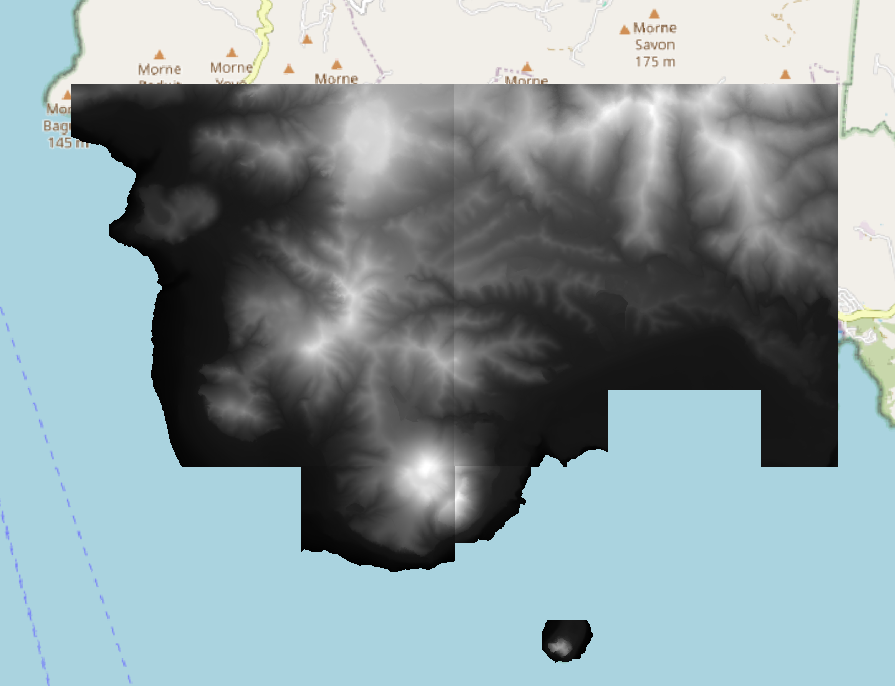
5. Merge the 4 tiles using the GDAL Merge tool.

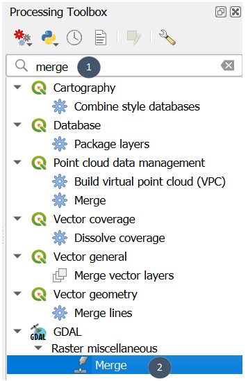
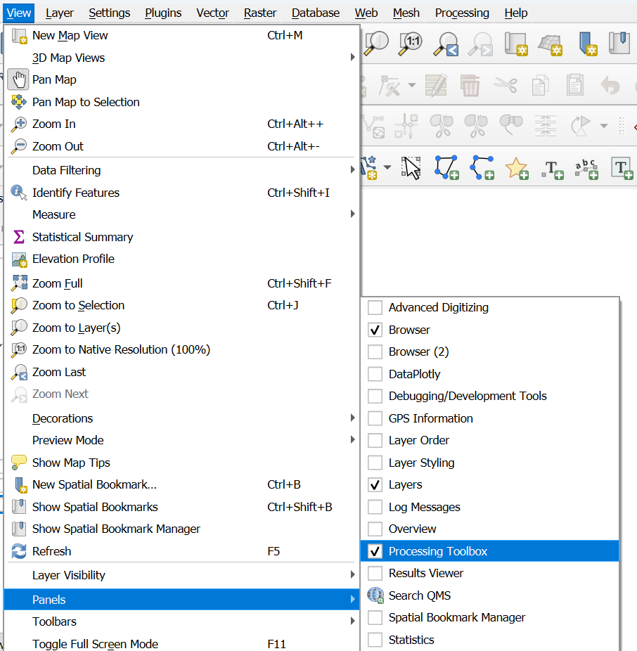
Tip

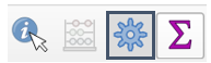
To display the Processing Toolbox panel if it does not appear in your workspace: View → Panels → Processing Toolbox. Or even easier: click on the gear icon just next to the sigma icon (top right a priori).

6. Fill in the inputs (marker 1) and save the output to a .tif file (marker 2) before running (marker 3).

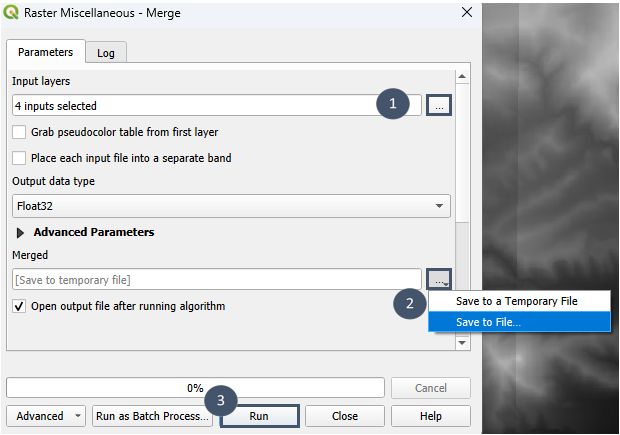
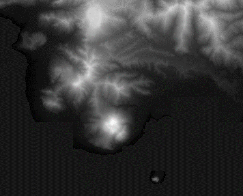
7. This process allows you to obtain a single DEM tile as output.

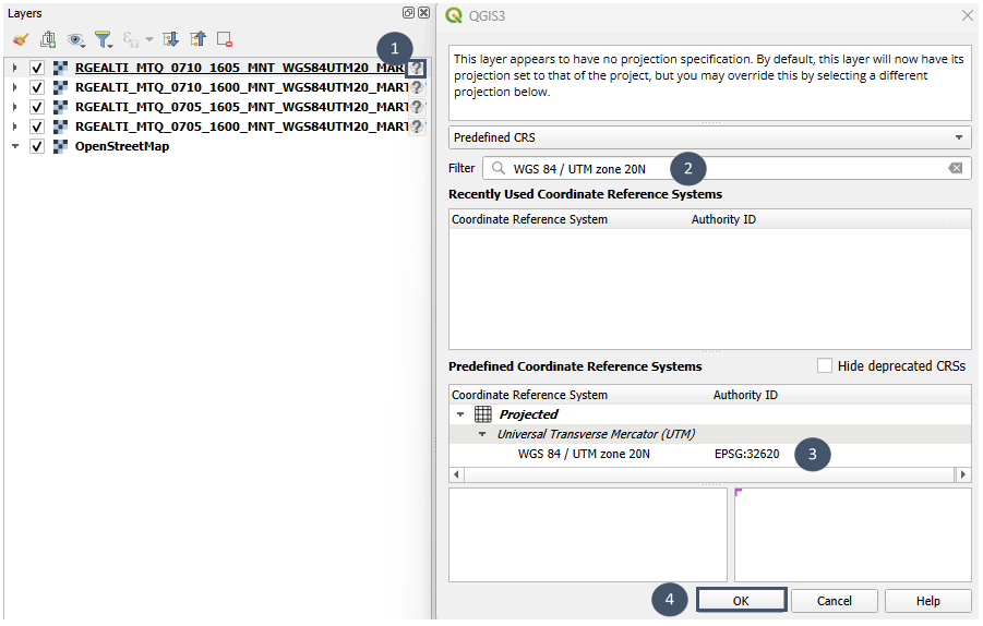
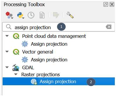
8. This tile is not georeferenced. To assign it a CRS permanently:

• Search for the Assign projection tool from GDAL in the Processing Toolbox (markers 1 and 2).

• Fill in the layer (marker 1) and the target CRS (marker 2), then Run (marker 3).

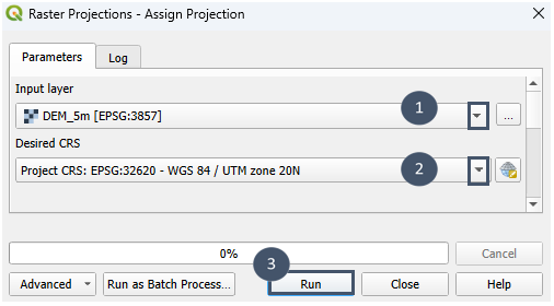
• Your initial layer is now georeferenced (no new layer created).

Tip

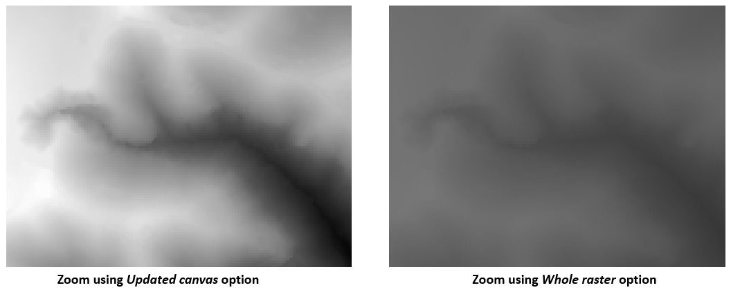
To have the DEM scale adjust automatically when you zoom in on the map:

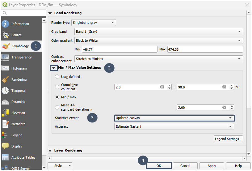
• Double-click your raster layer in the Layers panel.

• Choose Symbology in the window that opens (marker 1).

• In Min/Max Value Settings (marker 2), change the Statistics extent setting to Updated Canvas instead of the default Whole raster (marker 3).

Step 2: Specify possible discharge points (WWTP)

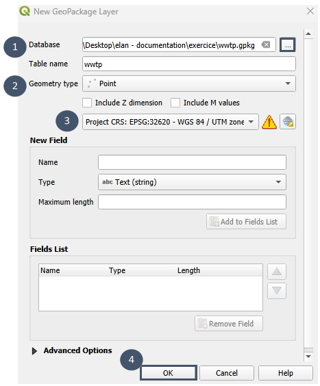
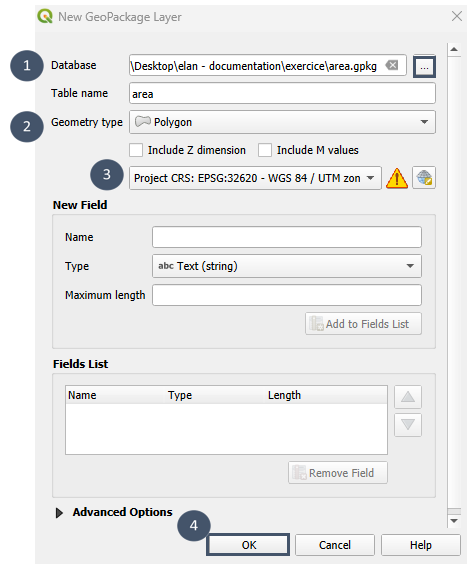
1. Create a new .shp or .gpkg layer.

2. Chose a storage location and name the layer (marker 1), then set its type to Point (marker 2).

3. For the CRS, choose the project CRS (here EPSG:32620 – WGS 84 / UTM zone 20N), then run (markers 3 and 4).

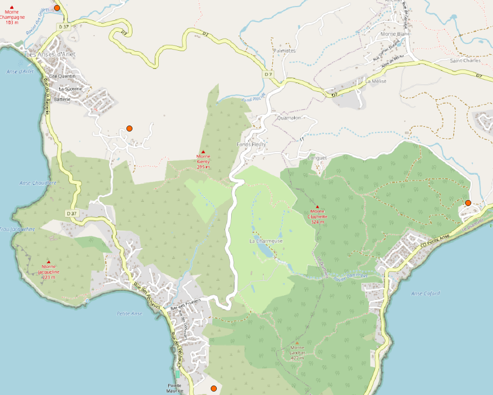
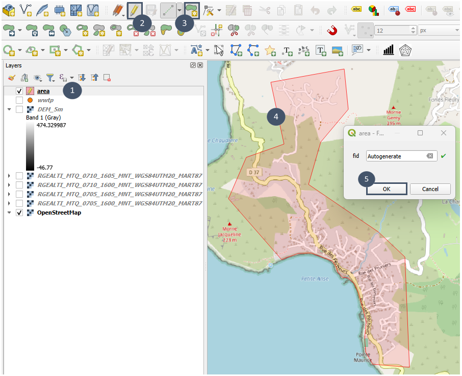
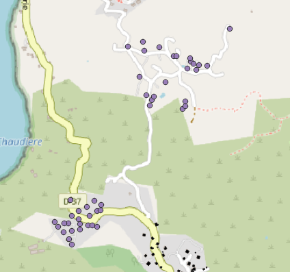
4. Add one by one the 4 possible locations following markers 1 to 5 as shown in the image.

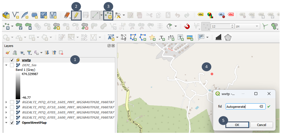
5. Be sure to save and disable edit mode once the 4 locations have been added.

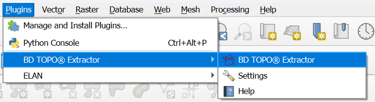
Step 3: Retrieve roads and buildings - using the IGN plugin (option 1)

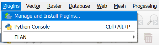
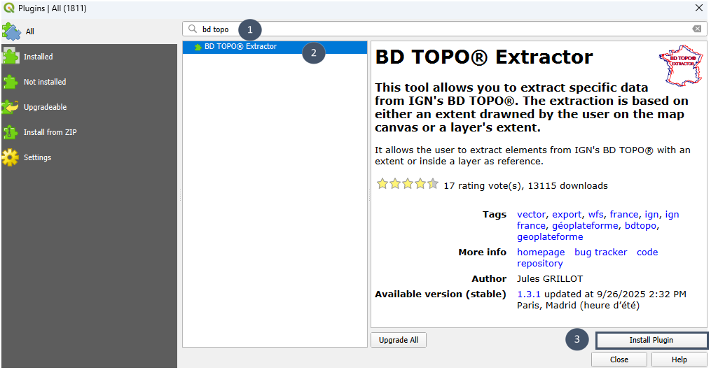
Prerequisite: Install the BD TOPO® Extractor plugin via the QGIS Plugin Manager.

Note

Data can also be downloaded directly from the IGN Geoservices website BD TOPO®, but a post-processing is then likely to be needed (data given at a department scale).

For buildings, only those in the area to be connected are needed. For possible roads, include those in the area plus those that connect to the two existing plants (see introduction).

Building retrieval

1. Create a new polygon layer in the project CRS.

2. Edit this layer and draw the area of interest.

3. Save and exit edit mode.

4. Launch the plugin.

5. Specify the layer of interest (marker 1), tick Building (marker 2), and specify the output folder (markers 3 and 4) before clicking OK (marker 5).

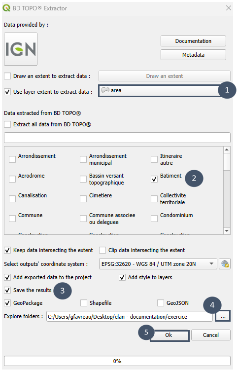
You will obtain an output like this:

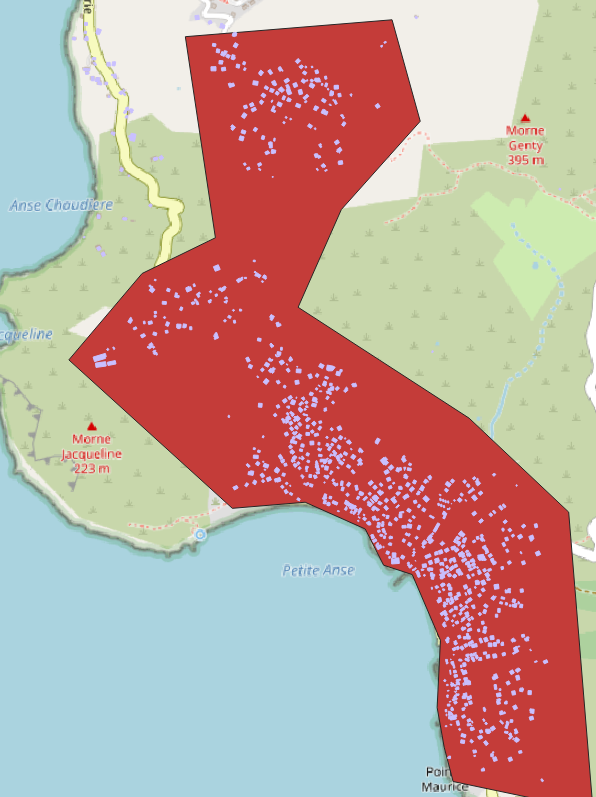
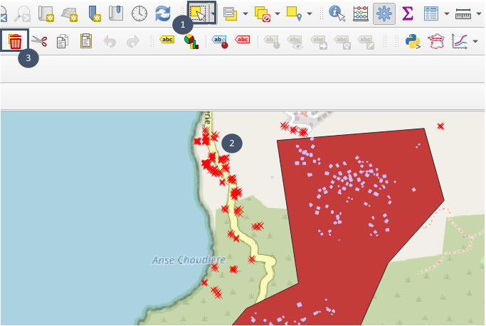
6. Edit the layer (pencil icon), select (markers 1 and 2), then delete the few entities located outside the area (marker 3). Save before exiting edit mode.

Road retrieval

1. Launch the BD TOPO® Extractor plugin.

2. Delimit the area to extract on the map (markers 1 and 2), tick Tronçon de route (marker 3), and specify the output folder (markers 4 and 5) before clicking OK (marker 6).

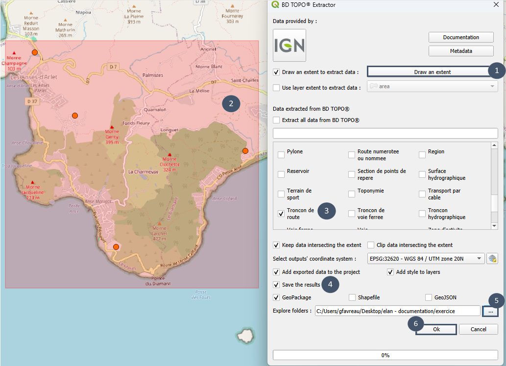
You will obtain an output like this:

Post-processing of layers

The layers can then be edited as needed. For example, in this case, restrict usable roads by removing footpaths.

Editing allows the user to transcribe its field knowledge (roads that cannot be used, or conversely, adding possible paths, fine selection of buildings to connect or not) and therefore contributes to obtain more relevant results.

Step 3: Retrieve roads and buildings - using Elan (option 2)

Building retrieval

By applying the Roads and Buildings module <routes> to the area defined earlier, the following outputs are obtained for buildings:

Road retrieval

By applying the module to an expanded area to include possible connections to the existing treatment plants, you will obtain an output of this type:

Post-processing of layers

The layers can then be edited to reflect your field knowledge (roads that cannot be used or, conversely, adding possible paths, fine selection of which buildings to connect). This step helps improve the relevance of the results obtained from the Sewer network module.

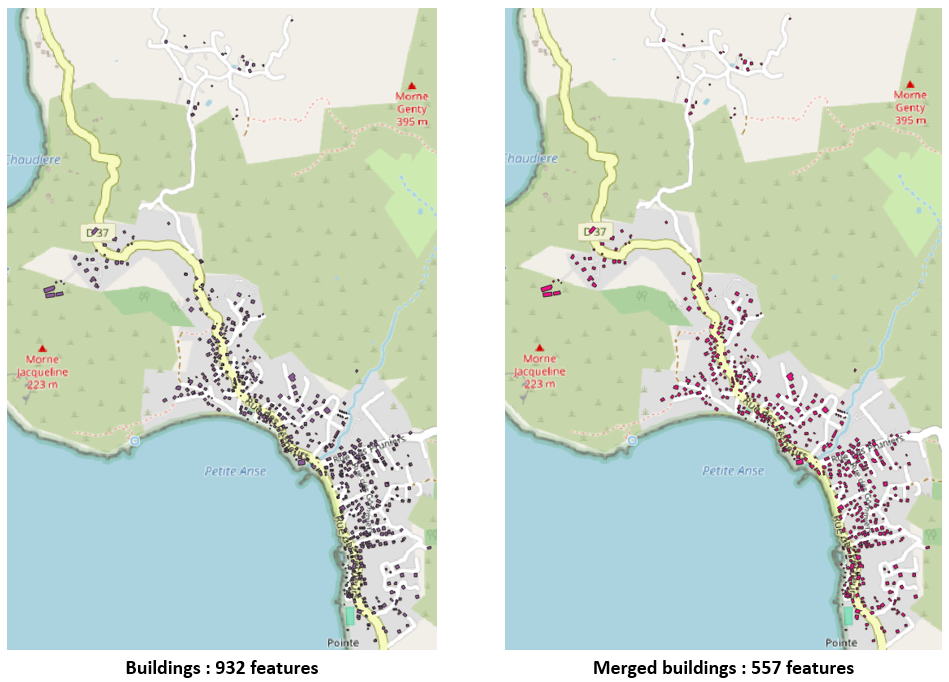
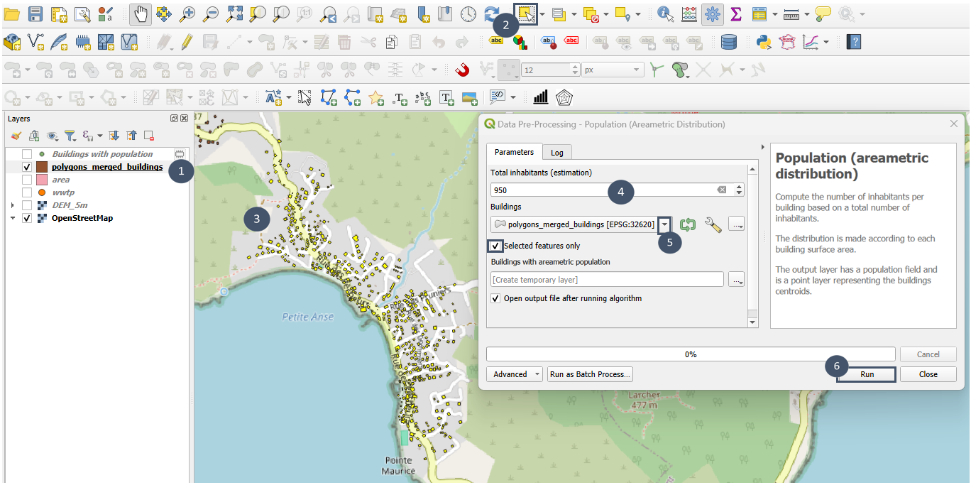
Step 4: Distribute population among buildings and reduce polygons to their centroids

The population of Petite-Anse is estimated at 1,100 inhabitants, with 150 in the upper area and 950 in the lower area.

In this example, population will be distributed according to an areametric distribution: the number of inhabitants associated to each building depends of its footprint. Therefore, we will use the module Population (areametric distribution) and not the module Population (uniform distribution).

Prerequisite: A polygon layer containing the buildings to be connected, obtained with the Roads and Buildings module and post-processed (removal/addition of certain buildings according to field knowledge of the area).

• Population distribution in the upper area

1. Select the buildings in the upper area (markers 1 to 3).

2. Launch the Population (areametric distribution) module as explained here.

3. Enter 150 for the Total inhabitants of the area (marker 4), tick Selected features only after selecting the building layer (marker 5), then run (marker 6).

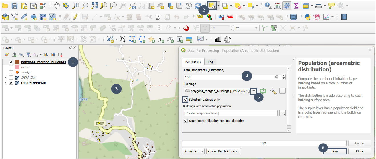
4. You will obtain the following layer.

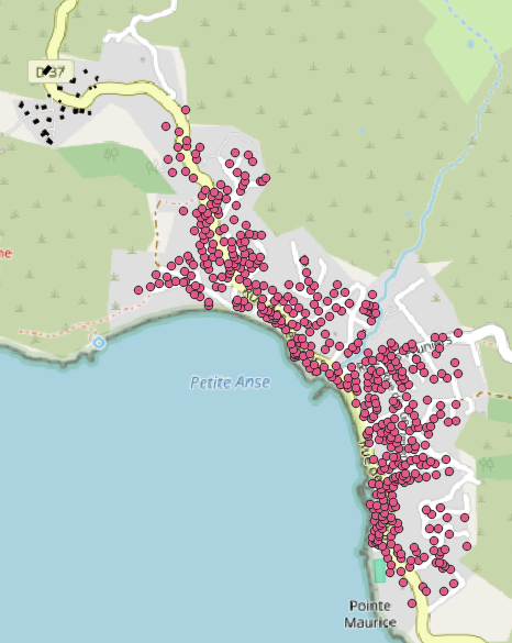
• Population distribution in the lower area

1. Repeat the same procedure, this time selecting the lower area and entering 950 for the Total inhabitants of the area.

2. You get the following layer.

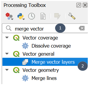
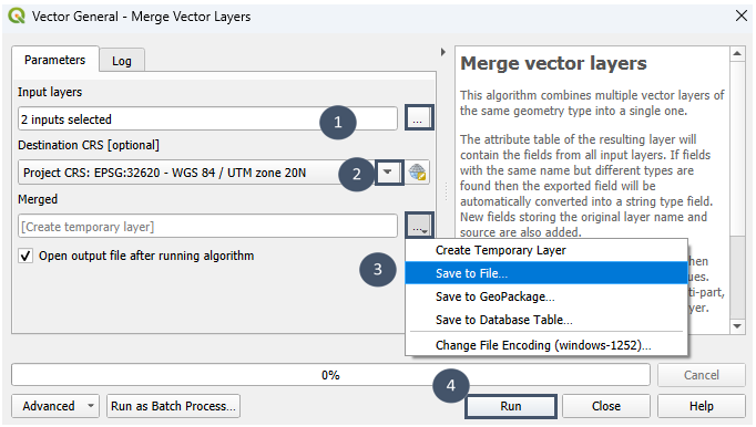
• Merging the two output layers

1. In the QGIS Processing Toolbox, search for Merge vector layers.

2. Select the two layers (marker 1), choose the project CRS (marker 2), set the output file (marker 3), then run (marker 4).

Viewing the attributes of the resulting layer:

Select the layer (marker 1) and open the attribute table (marker 2).

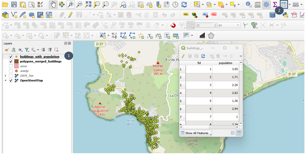
The resulting layer contains the centroids of buildings in both the upper and lower areas, and for each centroid, the population attribute is filled in. This layer complies with the conditions to be used as input for the Sewer network module.

Note

The geopackage entrees_reseau.gpkg given in the following section includes several layers:

• buildings_osm_population was generated following these steps: Roads and buildings module, manual post-processing (finer selection of buildings to connect), Population (areametric distribution) module;

• buildings_ign_population was obtained using BD TOPO® Extractor plugin, then applying a manual post-processing and finally using the Population (areametric distribution) module;

Both layers can be used as inputs for the Sewer network module. The layer based on IGN data contains more buildings (best data quality) and thus will a priori provide more relevant results.

• roads_reduced_area results of the use of the Roads and buildinds module on zone _reduite layer (in zones.gpkg) followed by a manual post-processing (elimination of impassable roads);

• roads_enlarged_area was obtained using the Roads and buildings module on zone _elargie layer (in zones.gpkg) and then a manual post-processing (elimination of impassable roads);

• wwtp that contains the 4 possible locations for wastewater treatment plants.

The geopackage intermediate_layers.gpkg contains all intermediate layers that were necessary to obtain these 5 layers.

Create a scenario

Step 1: Pre-designing the sanitation sewer network (Sewer network Module)

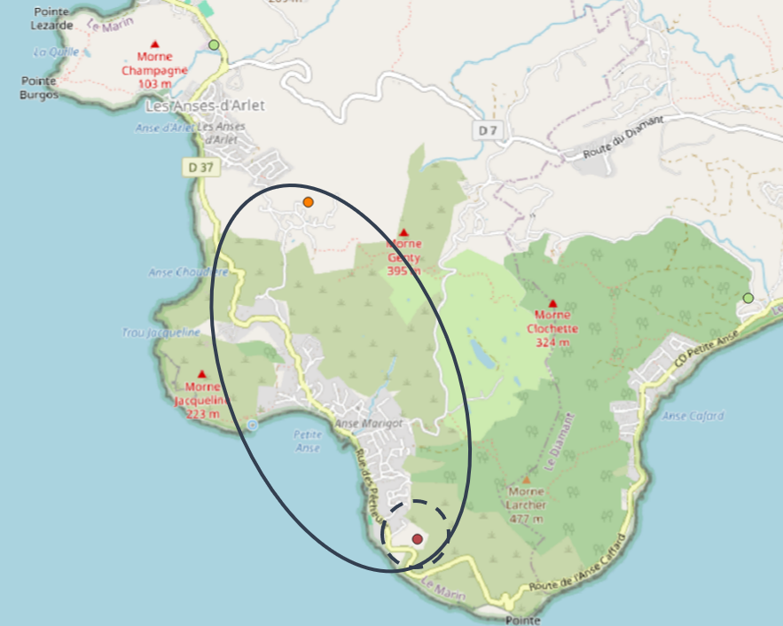
The scenario we will create in this step-by-step guide will consider connecting the area to one of the possible discharge point locations: the southern one.

Note

To reproduce this step-by-step example, you can either use the data you prepared by following the previous section, or download the data here.

1. Using the Sewer network module

• Select the southern WWTP (markers 1 to 3).

• Search for elan in the Processing Toolbox (marker 4) and select Sewer network (marker 5).

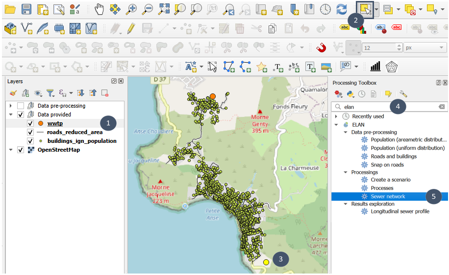
• Specify the 4 geographic layers (markers 1 to 4). Be sure to tick Selected features only to consider only the WWTP in the south of the area.

• Check if the population attribute of the building layer was correctly self-detected for the Population (field) input (bottom insert).

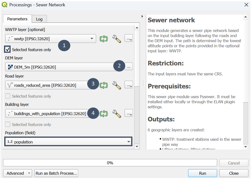
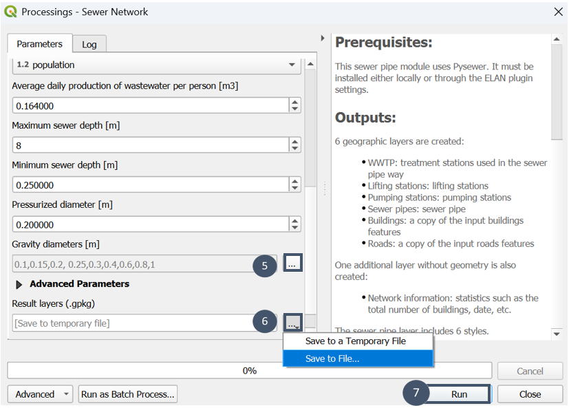
• Leave the default values for the various technical parameters.

• Select all possible options for gravity diameters (marker 5).

• Choose a name and a saving location for the file (marker 6).

• Run (marker 7).

2. Results from the Sewer network module

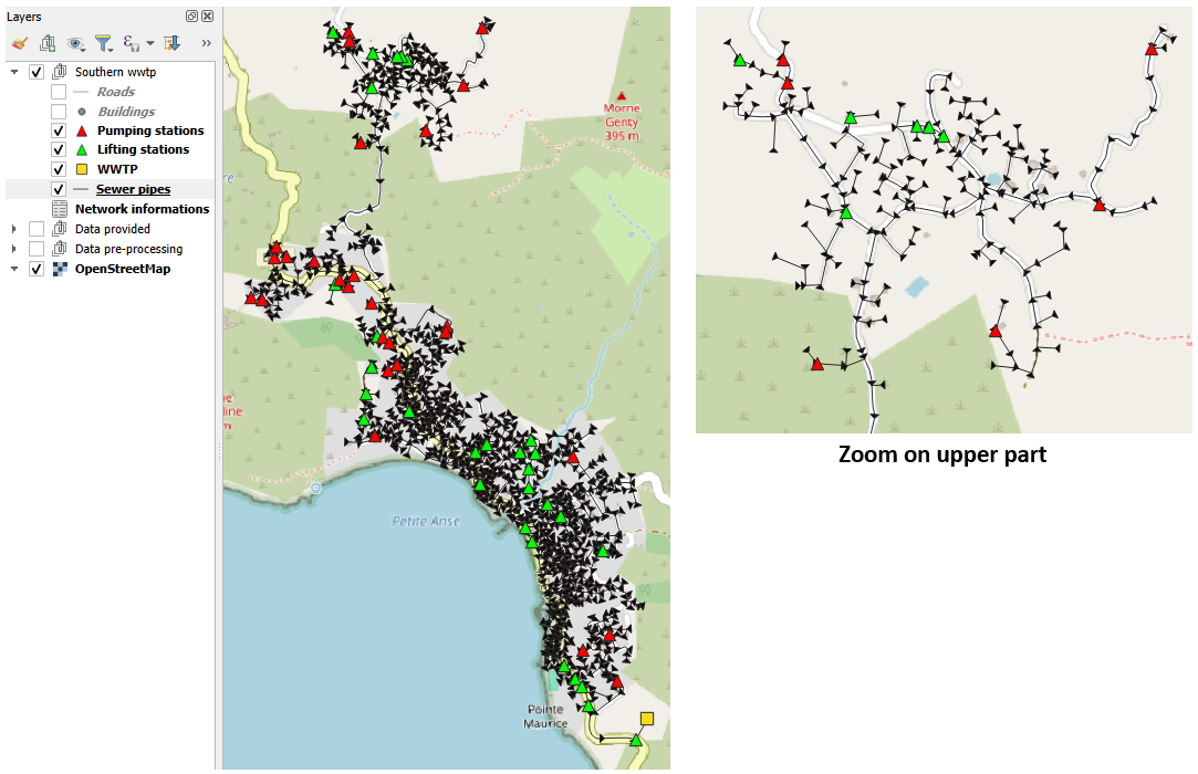
After executing it, you will obtain the following view:

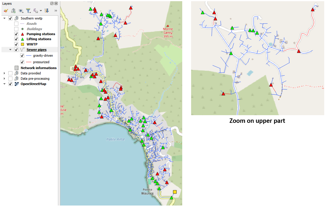
Note

Layers relative to roads and buildings do not appear in this view and the following ones for more clarity.

6 geographic layers have been loaded into your workspace, each one with its own symbology:

• yellow square for the WWTP

• random colored lines for roads

• random colored points for buildings

• green triangles for lifting stations

• red triangles for pumping stations (private and non-private)

• blue lines for gravity-driven sections and red lines for pressurized sections

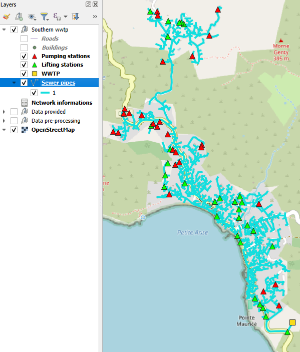
Other styles are available for the Sewer pipes layer. To access them:

1. Select the Sewer pipes layer and right-click.

2. Go to Styles.

3. Select the style of your choice among the 5 alternatives provided.

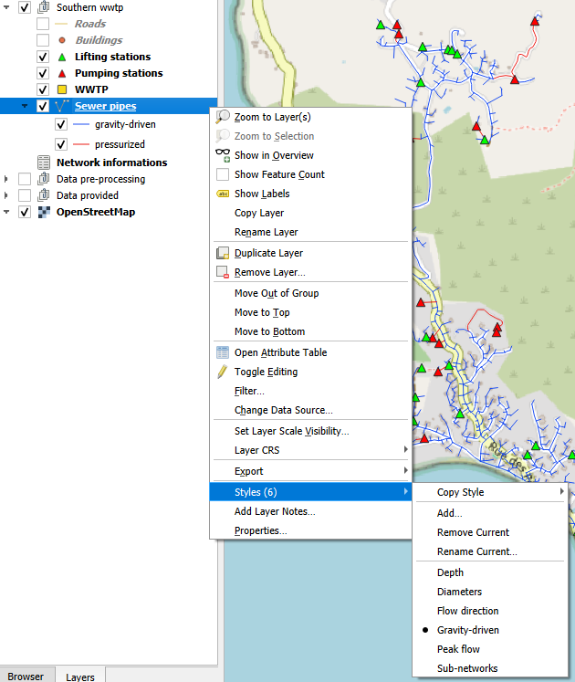
Diameters style

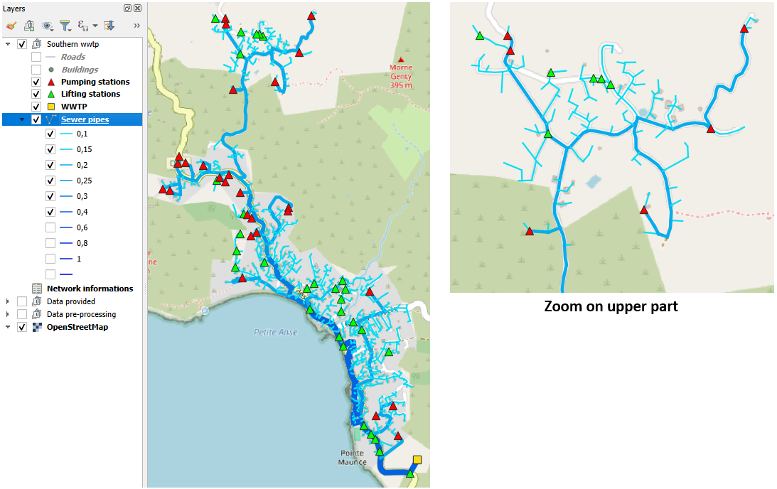
Tip

To know exactly how many features fit each diameter: right-click on Sewer pipes and tick Show Feature Count. You will get something of this kind:

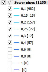
This tip can be applied to any vector layer.

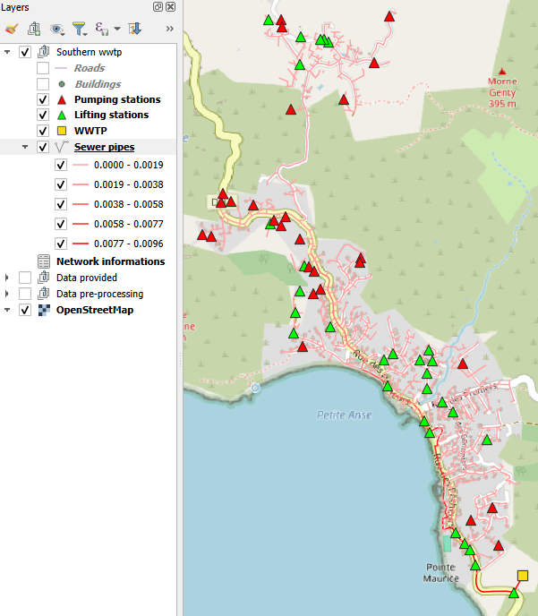
Peak flow style

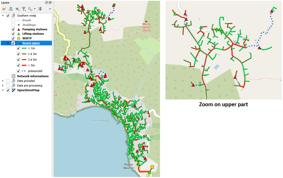
Depth style

Flow direction style

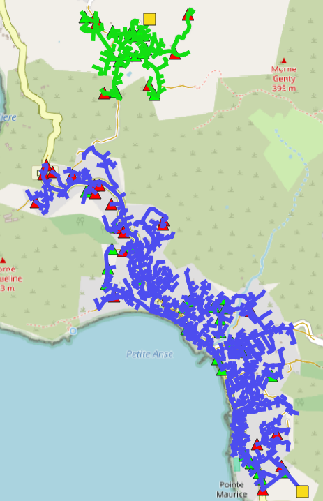
Sub-networks style

Note

The Sub-networks style is uniform here, since this scenario considers a single treatment plant, therefore a single sewer network (no sub-networks). Considering 2 discharge points, a view of this kind would be obtained:

Tip

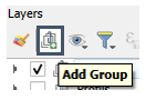
To organize your workspace with the different layers, you can create groups (e.g., Data Pre-processing, Data Provided, and Sewer Network - Southern WWTP).

To do this, simply click the Add Group icon and drag the layers you want to group into it.

3. Consulting the Network information layer and attributes of other layers

• Select the Network information layer (marker 1).

• Click on the Open attribute table icon (marker 2).

• A window opens giving you access to all the information in the layer (marker 3).

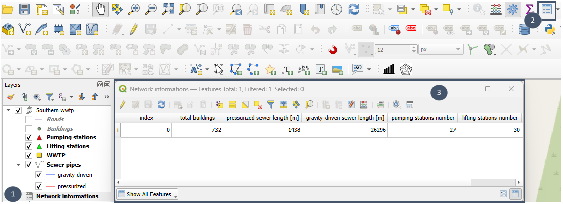
To consult the attributes of the other 4 layers produced by the module, proceed the same way by selecting the layer whose attributes you want to view.

The full list of attributes available for each layer is detailed here.

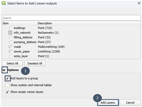
Tip

If you have to load the geopackage containing the 7 layers in another project, you can directly load it into a common group following these steps:

• Drag and drop the .gpk from Browser to the map canvas.

• In the window that opens, pull down Options and tick Add layers to a group (marker 1).

• Click on Add Layers (marker 2).

  

Results exploration (Longitudinal sewer profile module)

To explore the preliminary sizing proposed by the Sewer network module, you can view the underground profile of a sequence of pipes using the Longitudinal sewer profile module coupled with the QGIS Elevation profile tool. An example is given in the general documentation.

Step 2: Preliminary sizing of the WWTP(s) (Processes module)

1. Adjusting inflow concentrations in the WWTP layer

The WWTP layer obtained after running the Sewer network module has several attributes. Among them the inflow concentration of each pollutant. In this example, we will keep the default pre-filled values, i.e.:

• TSS: 288 mg/L

• BOD₅: 265 mg/L

• TKN: 67 mg/L

• COD: 646 mg/L

• NO₃-N: 3 mg/L

• TP: 9.4 mg/L

• e.coli: 0 UFC/100mL

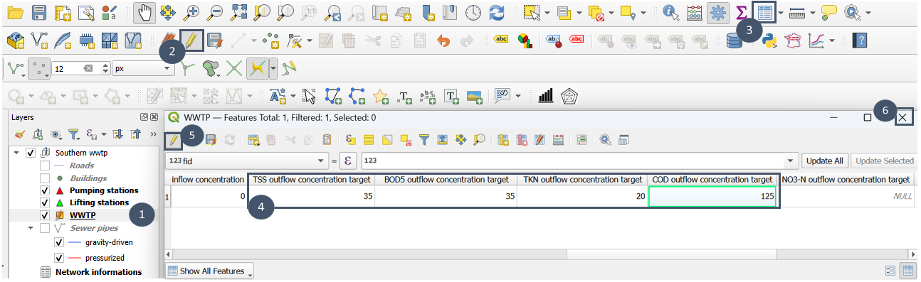
2. Specifying outflow concentration targets in the WWTP layer

The outflow concentration targets to be met for a plant located south of the area are as follows:

• TSS: 35 mg/L

• BOD₅: 35 mg/L

• TKN: 20 mg/L

• COD: 125 mg/L

• Select the WWTP layer (marker 1).

• Switch to edit mode (marker 2) then open the attribute table (marker 3).

• Fill the numerical values indicated for TSS, BOD₅, TKN, and COD (insert 4).

• Exit edit mode (marker 5) and close the attribute table (marker 6).

3. Delimiting the available surface area (optional)

• Create a new polygon layer (.gpkg or .shp).

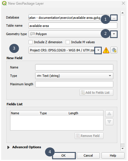
• Edit the layer and delineate the available surface area.

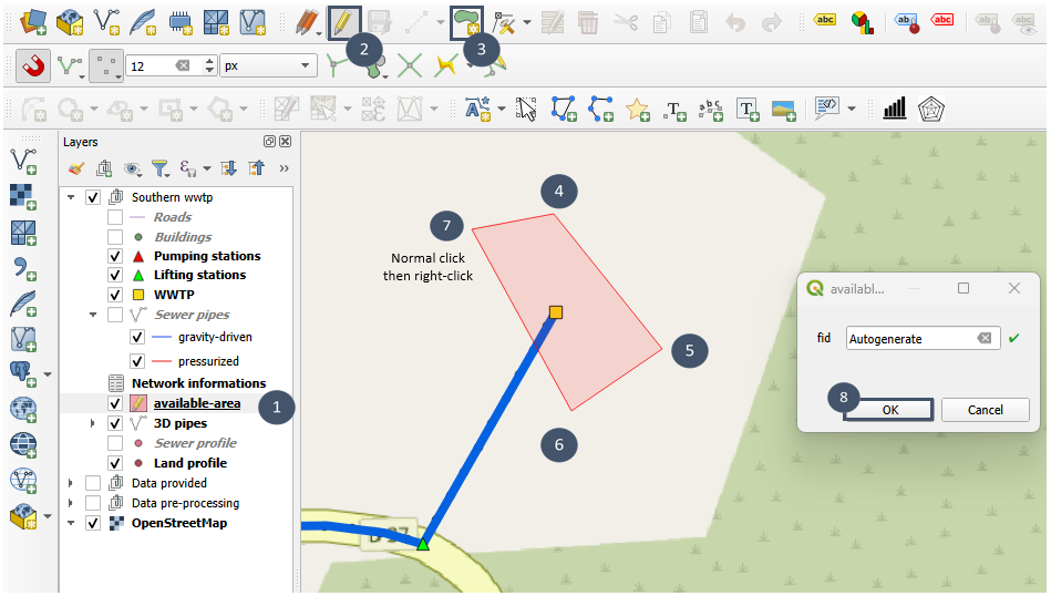
• Save and exit edit mode.

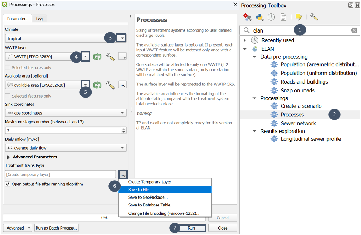
4. Using the Processes module

• Search for elan in the Processing Toolbox and select Processes (markers 1 and 2).

• Choose Tropical for climate (marker 3).

• Indicate the WWTP layer where you filled in the attributes (marker 4) and the available-area layer you just created (marker 5).

• Verify that the fields identified for GPS coordinates and daily inflow are correct.

Note

You can also check if inflow concentration and outflow concentration target fields were correctly self-detected unfolding Advanced parameters.

• Provide a name and save location for the output file (marker 6), then run (marker 7).

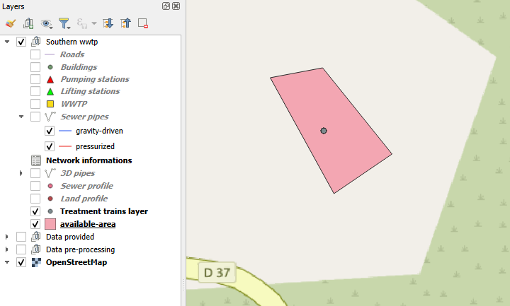
5. Exploring the characteristics of pre-sized treatment trains

After execution, you obtain a point layer output of this type:

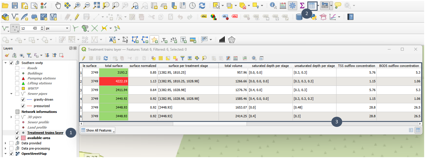
To access the attributes of this layer:

• Select the Treatment trains layer (marker 1).

• Click the Open attribute table icon (marker 2).

• A window opens giving you access to all the information in the layer (marker 3).

Step 3: Pre-selecting a treatment train for the discharge point

To help you to pre-select a treatment train, you can display graphical représentations (radar plot and bar plot) where all possible treatment trains for this discharge point are represented (see here for more details).

Radar plot

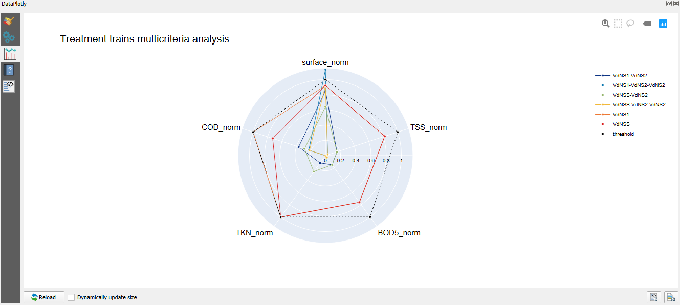
Here, 6 treatment trains meet the required outflow concentrations (deviations in green in the attribute table, dots below threshold 1 on the radar plot):

• VdNS1-VdNS2

• VdNS1-VdNS2-VdNS2

• VdNSS-VdNS2

• VdNSS-VdNS2-VdNS2

• VdNS1

• VdNSS

The total surface appears in red for the VdNS1–VdNS2–VdNS2 train (attribute table) as it exceeds the available surface area (dot above threshold 1 on the radar plot).

Bar plot

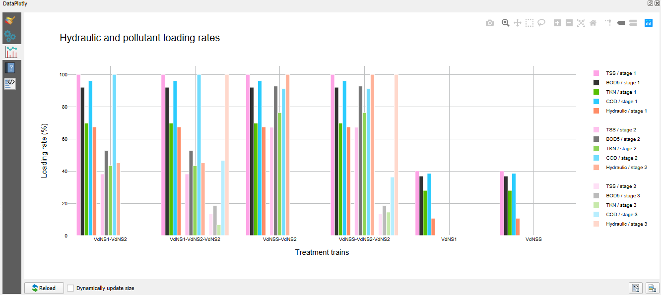
The single-stage treatment trains (VdNS1 and VdNSS) here are sufficient to meet the outflow concentration targets and are generally less costly than multi-stage treatment trains. Given the pollutant loading rates and the hydraulic loading rate, they could be two promising treatment trains options.

A first scenario could therefore be: the sewer network obtained in step 1 coupled with a VdNS1 train. Pairing it with a VdNSS train could form a second scenario.

Step 4: Creation of a scenario item (Create a scenario module)

Once you have identified the sewer network/treatment trains coupling for a scenario, you can create a scenario item using the Create a scenario module as detailed in global documentation. This item will then be useful to assess this scenario and compare it to other possible scenarios.

Exercise: Creating a second scenario for Petite-Anse

To practice the content of this page, you can try following the same steps, but this time considering 2 possible discharge point locations: one in the South of the area and one in the North.

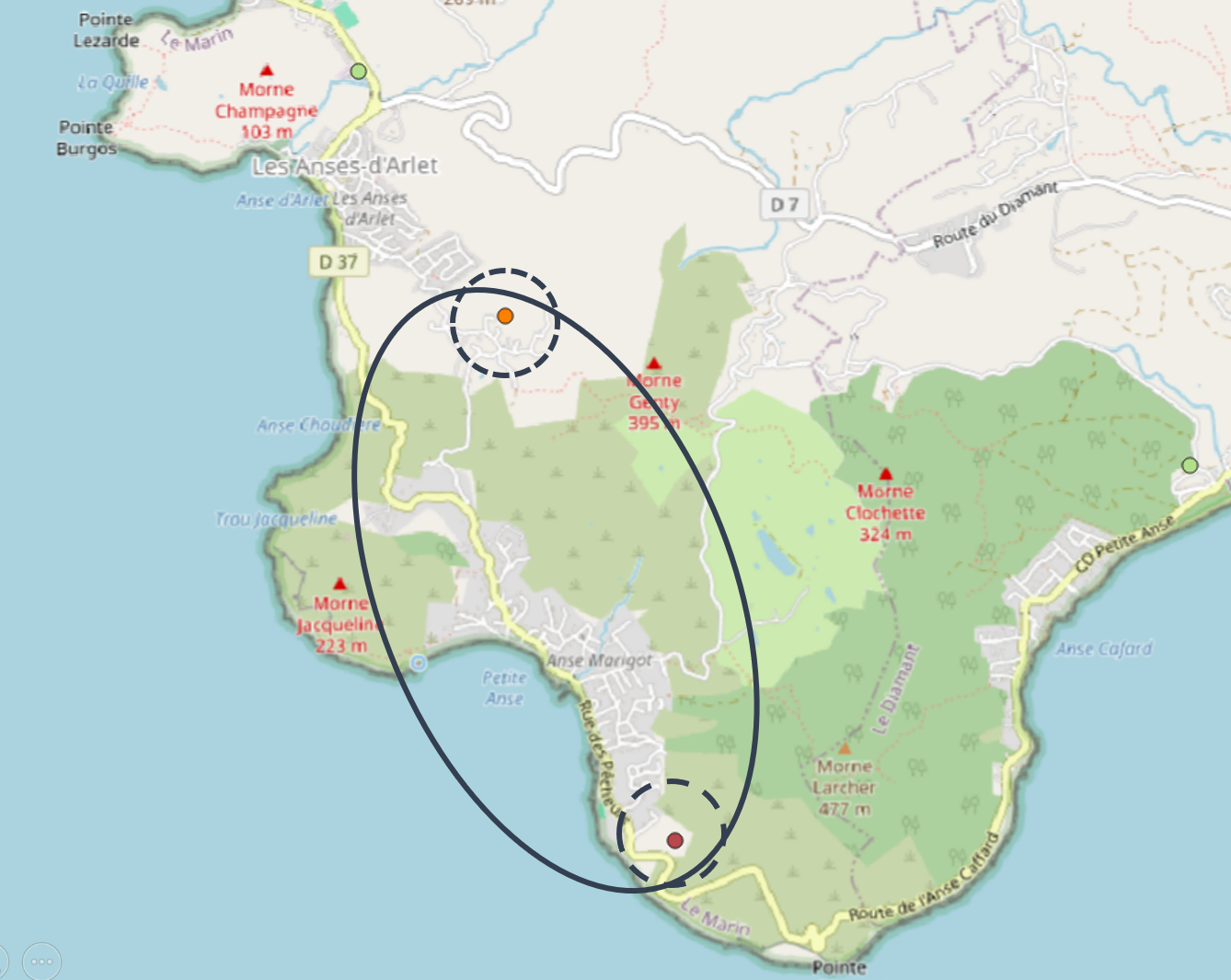
The outflow concentration targets for the northern location are less strict (no nitrogen constraint):

• TSS: 35 mg/L

• BOD₅: 35 mg/L

• COD: 125 mg/L

Important

The iterative nature of scenario definition is not detailed in this step-by-step, but it is a possible practice (if not unavoidable).

For example: if you find that some buildings are too “costly” to connect (more than 40 meters of pipe for one building), you can edit the buildings layer and remove them to assess the impact of leaving them on on-site sanitation on the pre-sized sewer network. Similarly, you can adjust possible roads by deleting and/or adding some.